EMAFD has developed a six degree of freedom (6-DOF) for more serious precision shooters that would like to have more accurate solution for Extreme Long Range (ELR).  ELR being defined as taking the projectile to its limiots within the transonic and subsonic range.  Due to the complexity and amount of aerodynamic data required this solution is only available on individual cases.  Structural data (inertia’s) are obtained from a CAD drawing and aerodynamics data (Cd,Cl,Cm etc) are obtained from a very high definition CFD model.  Aerodynamic data is obtained from the supersonic, transonic and  subsonic range.  At the present time, EMAFD is working on the CFD data for the Hornady 6.5 mm ELD Match 140 gr.

Below, the work used for validation of the 6-DOF is presented.

============================================================================                                               6-DOF Simulation of Firearm Trajectories

by Ange (Phil) Du, Advisor: Dr. JM Dhainaut

Introduction

This study aims to simulate projectile trajectories of firearms with a six-degree-of-freedom (6-DOF) model. Most of today’s ballistic calculators are based on the method of point mass trajectory. Such method requires limited computing power and only a few parameters input by the user. However, as its name suggests, it models the projectile as a simple point, neglecting its shape and attitude, leaving potentially significant aspects out of the equation. The 6-DOF method explored in this study models the entire projectile throughout the simulation. This allows for two potential outcomes: 1. a more accurate trajectory compared to point mass methods (6-DOF simulation as a more advanced ballistic calculator), and 2. revealing more details in the motion of a projectile that point mass methods cannot provide.

Methodology

The 6-DOF model developed in this study is based on Ballistics: theory and design of guns and ammunition, by Carlucci and Jacobson (2008). With changes and optimization made for computer simulation. MathWorks MATLAB R2019a is the platform to perform the ballistic simulation numerically. The main MATLAB function for the simulation is ODE45. A copy of the MATLAB code is provided alongside this document. To compare against the 6-DOF simulation result with point mass trajectory, JBM Ballistics, a popular web-based ballistic calculator is used. Two types of bullet are simulated in this study: Hornady 6.5mm 140gr ELD-Match and M855 5.56x45mm NATO.

Terminologies

Compared to ordinary physics analysis, some terminologies used in ballistic studies, ballistic data published by manufactures and range cards output by ballistic calculators can look similar while denoting different properties. This section denotes to illustrate such differences to reduce any potential confusion by readers.

X, Y, Z vs. Range, Drop, Windage

Figure 1: Relationship between X, Y, Z and Range, Drop, Windage

In a Cartesian coordinate, the x, y and z axes represent three directions perpendicular to each other. Such a system is used in during MATLAB simulation, with x-axis pointing at the initial firing azimuth, parallel to ground (sea level). Y-axis is pointing vertically upward, perpendicular to the ground and away from the earth center. Z-axis represents sideway distance, with shooter’s right being positive. However, unlike x-axis, “range” on a range card is not the horizontal distance forward, but rather measured along the firing line-of-sight. For example, if the firearm is pointing 30° upward, 200m in range is only 173.2m away horizontally from the firing position. “Drop” at certain range is the distance that the bullet has fallen below the line-of-sight (or above if before zeroing range), but not the x-axis. Windage and z-axis can mostly be treated the same. It should also be noted that “windage” is an umbrella term that represents not just crosswind but the sum of all sideway movements, including those due to Magnus Effect, Coriolis Effect, aerodynamic jump etc. Figure 1 above shows the differences between these coordinate systems.

Yaw vs. Angle of Attack

In aviation terms, pitch and yaw describes the up/down and sideway angle of an object, while “angle of attack” refers to the angular difference between its longitudinal axis and velocity vector. However, in ballistic studies, some authors like to use “yaw” (or “total yaw”) in place of angle of attack. This may be okay in point mass trajectories, but can cause some ambiguity in 6-DOF, as the pitch and yaw angle of a bullet are also studied. Thus, the code and discussion of this study will stick to the unambiguous term “angle of attack” or “AoA”.

Partial 6-DOF Simulation Results

Before developing a full 6-DOF simulation, the model is tested with only drag being the main factor of the simulation, with wind and Coriolis Effect being optional. Lift and other rotational motions are not considered. The drag coefficient in this case is calculated based on G1 or G7 functions at different Mach number. The user only needs to supply the ballistic coefficient, mass, dimensions and muzzle velocity of the bullet, all of which are either available from the manufacturer of easily measurable. The Hornady 6.5mm 140gr bullet is used in the following simulation, with ballistic data from Ballistic Performance of Rifle Bullets by Litz (2017).

Figure 2: Drop, Velocity and Windage of Partial 6-DOF Simulated Hornady 6.5mm 140gr, Flat Firing with no Wind, Compared with JBM Point Mass Trajectory

Figure 2 shows the simplest scenario: flat firing with no wind or Coriolis Effect factored in. The 6-DOF simulation in this case is very similar to the simple point mass trajectory. The 6-DOF code does considers more environmental factors, namely change of air density at different altitude (code provided by Dr. Dhainaut) and change of speed of sound due to this. However, the results are still close. By comparing table 1 and 2, one can see that the 6-DOF simulation and simple point mass only show a 0.2 MOA difference at 500m.

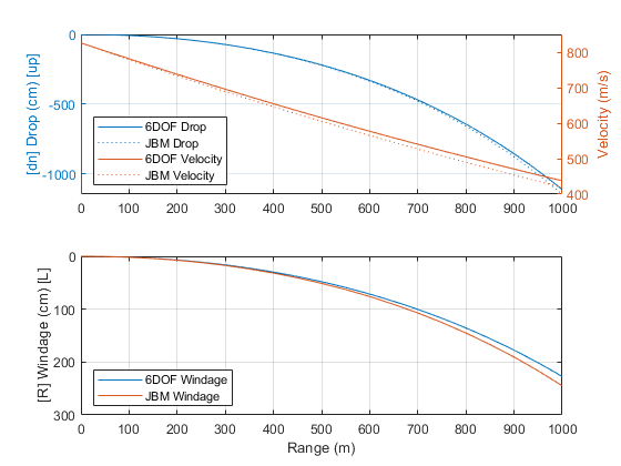
Figure 3: Drop, Velocity and Windage of Partial 6-DOF Simulated Hornady 6.5mm 140gr, 5m/s Crosswind to the Right, Compared with JBM Point Mass Trajectory

Compared to point mass methods, the 6-DOF approach can consider wind natively throughout the simulation instead of adding it in at the end. Figure 3 above shows the trajectory comparison when a 5m/s crosswind is blowing to the shooters right. The results again agree with each other, with windage at 500m only differs by 0.2 MOA according to table 3 and 4.

One advantage of the 6-DOF method of incorporating wind vector in the simulation in real time is that potentially wind can be written as a function of time or distance and not limited to 2D directions, allowing the simulation of more complicated scenarios such as wind gust, varying wind speed/direction along the flight path (a relevant situation in long range shooting) or rising air.

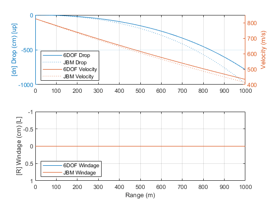
Figure 4: Drop, Velocity and Windage of Partial 6-DOF Simulated Hornady 6.5mm 140gr, Downhill 45° with 5m/s Uphill Headwind, Compared with JBM Point Mass Trajectory

To illustrate the 3D vector advantage of the 6-DOF simulation, a scenario of firing down a 45-degree hill, with 5m/s headwind blowing uphill along the slope is simulated. The point mass trajectory, however, does not consider any upward air movement. A significant difference in bullet drop can be seen in Figure 4, which according to Table 5 and 6, is over 2.5 MOA at 500m.

Coriolis Effect, the change in trajectory cause by Earth’s rotation, can also be simulated with 6-DOF. This effect is not considered in the simple point mass trajectory but available in modified point mass trajectory. Figure 5 shows the influence of Coriolis Effect on windage when firing direct North at 30°N latitude, under no wind condition. The result matches the modified point mass trajectory by JBM under the same condition. Magnus Effect is not enabled in the modified point mass trajectory.

Figure 5: Drop, Velocity and Windage of Partial 6-DOF Simulated Hornady 6.5mm 140gr, Coriolis Effect at 30° North, Firing North, Compared with JBM Modified Point Mass Trajectory

Full 6-DOF Simulation Results

One major obstacle in developing a fully modeled 6-DOF simulation is the lack of data on the aerodynamic coefficients need for the calculation. Compared to previous section, where only drag coefficient is needed, easily obtainable by publicly available ballistic data, full 6-DOF requires coefficients related to lift, spin and pitch damping, overturning and Magnus Effect. Even when neglecting some of the forces and moments that are too small to affect the simulation, a total of 8 coefficients are used. As the data for these coefficients are not available for the Hornady 6.5mm in the previous section, the projectile used in these simulations changed to M855 5.56mm NATO. This allows for incorporating the experimentally determined coefficients by Silton and Howell (2010) and McCoy (1985) (for subsonic region not measured by Silton).

Figure 6 below and table 9, 10 shows the full 6-DOF simulated trajectory with no initial angle of attack when compared to that generated by the modified point mass trajectory using JBM. Although this firing condition is without wind or Coriolis Effect, both methods show significant windage. Such side drift is due to the Magnus Effect as a bullet spins in the air with a non-zero angle of attack. This effect is neglected in the simple point mass trajectory but can be quite influential as discussed later. Note that since G7 ballistic curve is used in the JBM calculation, it produces a very low drag coefficient (0.075) below Mach 1 (at around 700m). This causes the bullet to almost stop decelerate beyond such point on the JBM trajectory. The 6-DOF simulation however uses the experimentally measured drag coefficient, which at this point retains a relatively large value (0.29). In reality, a 5.56mm bullet at this point would have already destabilized enough to induce a significant angle of attack, leading to a large drag coefficient. This phenomenon will be further discussed below.

Figure 6: Drop, Velocity and Windage of Full 6-DOF Simulated M855 5.56mm, Compared with JBM Modified Point Mass Trajectory Calculator

The above simulation assumes zero initial angle of attack, which requires perfectly balanced barrel and ammunition and is rarely the case in real life. The yaw and pitch angle shown in Figure 7 below indicate that the bullet only start to show signs of destabilization after 700m.

Figure 7: Longitudinal Axis Direction of Full 6-DOF Simulated M855 5.56mm, with No initial Aerodynamic Jump

In modified point mass trajectory, aerodynamic jump only results from the existence of wind upon bullet exiting the barrel, as it assumes that the bullet would exit pointing straight ahead.  However, as observed by Silton and Howell (2010), the M855 bullet in their experiment often exit the barrel with an angle around 2~4 degrees. Such an initial angle would cause an aerodynamic jump even without wind. The following 6-DOF simulations add a 3-degree initial angle in various directions to observe the effect on trajectory by such aerodynamic jump under no wind condition.

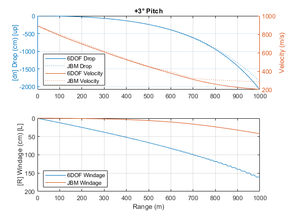
Figure 8: M855 5.56mm 6-DOF Simulation with 3° Initial Upward Pitch

Figure 9: M855 5.56mm 6-DOF Simulation with 3° Initial Downward Pitch

Figure 10: M855 5.56mm 6-DOF Simulation with 3° Initial Right Yaw

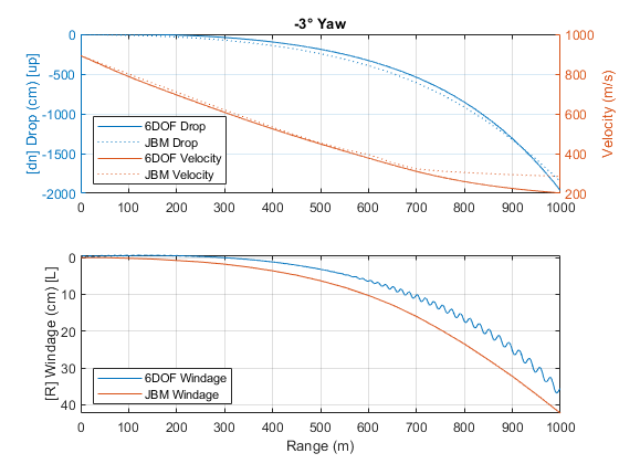
Figure 11: M855 5.56mm 6-DOF Simulation with 3° Initial Left Yaw

Figure 8 and 9 show that an initial angle in pitch would greatly affect, even invert the Magnus Effect side drift. An initial yaw angle does not affect side drift as much, but has a sizable influence on bullet drop (Figure 10 and 11), up to 5 MOA in this case (Table 13 and 14). These simulations help illustrate the difficulties in accurately predict the trajectory of a projectile by today’s ballistic computer: even if a model can precisely simulate a trajectory given the right initial conditions, some of the initial conditions themselves, like aerodynamic jump in this case, is unknown before firing, and only resulting from internal ballistic effects. The shooter may have a general idea of how well the bullets are stabilized upon exiting the muzzle, but the exact value and direction of the initial angle is very hard to predict.

An aerodynamic jump also significantly affects the stabilization of the bullet throughout out the flight. Carlucci in Chapter 8 of his book argues that the motion of a projectile contains two cyclic modes, fast and slow. This is observed by the experiment of Silton and Howell and support by this 6-DOF simulation, shown by Figure 12 and 13 below.

Figure 12: Longitudinal Axis Direction of Full 6-DOF Simulated M855 5.56mm, with 3° Aerodynamic Jump

Figure 13: First 100m of Figure X Zoomed In, Showing Both Slow and Fast Cyclic Modes

It can clearly be observed that the bullet exits the muzzle with both fast and slow cyclic modes. They both damp down to minimum before 400m. However, compare to experiment conducted by Silton and Howell, the simulated fast cyclic mode damps down sooner than slow mode. When comparing with previous zero aerodynamic jump simulation (Figure 7), the bullet in this case start to destabilize earlier: around 500m vs. 700m.

Conclusion

Contrary to the perceived outcome of this study, the 6-DOF approach appears not quite well-suited for being used as a more “advanced” ballistic calculator by itself. It is very demanding on computational power (30 seconds to several minutes of simulation time for 6-DOF compared to less than a second for other methods on an Intel Core i9 processor used in this study), yet the range cards it produces mostly do not differ practically from a simple point mass calculator within the effective range of the projectile (around 500 meter/yard for both 6.5mm and 5.56mm in this case) given the same input. However, it does clearly capture effects not covered by point mass trajectory methods, such as aerodynamic jump without wind and cyclic motions. This makes the 6-DOF simulation an optimal tool for ballistic study, with its results potentially improving other more computing-power-friendly ballistic calculators, and for projectile design. For example, if one aims to extend the effective range of the 5.56mm ammo, this 6-DOF simulation model can be used to test if a bullet design can significantly extend the distance where bullet starts to destabilize, before actual production.

It is also important to note that in a full 6-DOF simulation, one force or moment can only be neglected for being very small and non-influential (pitch damping force and rolling moment for example), but not for lack of data, as they are closely interdependent on each other. For example, lift depends on angle of attack, which itself results from overturning moment and pitch damping moment. If overturning moment is arbitrarily set to zero due to not knowing the corresponding coefficients, the rest of the simulation will fall apart. This makes full 6-DOF simulation very different from previous partial 6-DOF or point mass trajectory methods, in which one part of the computation (wind for example) can be safely disabled without affecting other factors (drag, Coriolis Effect, etc.) Thus, the full 6-DOF simulation is an “all or nothing” approach. If one cannot gather all the needed coefficients, they are much better off resorting to simpler approaches.